Simulating the Lennard-Jones fluid

This example will simulate a simple liquid that interacts via the Lennard-Jones pair potential:

\[u(r) = 4 \varepsilon \left[ \left(\frac{\sigma}{r} \right)^{12} - \left(\frac{\sigma}{r}\right)^6 \right]\]

The Lennard-Jones potential has two parameters: the energy \(\varepsilon\) and the size \(\sigma\).

First, we import relentless. We don’t need any simulation packages: relentless will take care of this for us.

import relentless

Model

Next, we setup the model. We will assign the type “1” to the particles. We create an instance lj of the Lennard-Jones potential. Then, we specify the parameters for interactions between particles of type 1 by updating the pairwise coefficient matrix lj.coeff:

lj = relentless.model.potential.LennardJones(types=("1",))
lj.coeff["1", "1"].update({
    "epsilon": 1.0, "sigma": 1.0, "rmax": 3.0, "shift": True
})

Here, we have chosen \(\varepsilon = 1\) and \(\sigma = 1\). We have also used rmax and shift options to truncate the potential to zero at \(3\sigma\), which is a common choice for the Lennard-Jones potential.

To finish specifying the model, we should also define the thermodynamic state, e.g., the number of particles, the volume, and the temperature. We can conveniently collect this data in an Ensemble:

state = relentless.model.Ensemble(
    T=1.5, V=relentless.model.extent.Cube(L=10.0), N={"1": 400}
)

Here, we have chosen to have \(N=400\) particles in a cubic box with edge length \(L=10\) at temperature \(T=1.5\). The units of \(L\) are implicit to the model (i.e., they are same as \(\sigma\)). The units of \(T\) are also partially implicit to the model (i.e., they are related to the units of \(\varepsilon\)) but can be manipulated through the Boltzmann constant \(k_{\rm B}\) that converts between energy and temperature units. By default, \(k_{\rm B} = 1\).

Simulation operations

We now need to specify our simulation protocol. relentless runs a simulation as a sequence of operations.

Every simulation protocol must have an initialization operation to set up the system. Here, we will initialize our system in a semi-random configuration. The diameters option will space out the particles to prevent overlap, so we set it equal to \(\sigma\).

init = relentless.simulate.InitializeRandomly(
    seed=42,
    T=state.T,
    V=state.V,
    N=state.N,
    diameters={"1": lj.coeff["1", "1"]["sigma"]}
)

After initialization, we can run a sequence of simulation steps. Our first simulation step is a short equilibration using Langevin dynamics:

eq = relentless.simulate.RunLangevinDynamics(
    steps=10000, timestep=0.005, T=state.T, friction=0.1, seed=2
)

Then, we will run a production simulation using Langevin dynamics. We attach an analysis operation to this step so that we can also write a trajectory trajectory.gsd of the particles:

dump = relentless.simulate.WriteTrajectory(
    filename="trajectory.gsd", every=2000
)

prod = relentless.simulate.RunLangevinDynamics(
    steps=50000, timestep=0.005, T=state.T, friction=0.1, seed=7, analyzers=dump
)

Running a simulation

Now that we have defined our operations, we can combine them to be run by a specific simulation engine. Here we will use HOOMD-blue to perform the simulation. In order to run this cell, you need to make sure you have the necessary dependencies installed, or you will get an error. Always make sure to check relentless’s documentation for the simulation engine you want to use for these!

sim = relentless.simulate.HOOMD(initializer=init, operations=[eq, prod])

We then need to prepare the model’s potentials for the run using relentless.simulate.Potentials. This object will turn one or more potentials, which are analytical functions in relentless, into a single tabulated potential that can be simulated. This means that you need to specify a few additional parameters for the tabulated potential (its starting point, stopping point, and number of subdivisions), along with the buffer that is used to construct pair neighbor lists in many simulation packages.

Notes: The starting point should be greater than zero because the Lennard-Jones potential diverges at \(r=0\). The stopping point should be sized based on where you would typically truncate interactions. Both the starting and stopping point must be fixed numbers so make sure that you choose them to be large enough or also remember to update them if you vary the potential parameters.

pot = relentless.simulate.Potentials()
pot.pair = relentless.simulate.PairPotentialTabulator(
    potentials=lj, start=1e-6, stop=3.0, num=100, neighbor_buffer=0.5
)

Last, we can run the simulation. An output directory is required for all runs, so here we will use the working directory. This will be the slowest step of this example, but don’t worry, it took less than a minute to run on an old laptop.

result = sim.run(potentials=pot, directory=".")

The result contains data from the run. Some of it can be useful for subsequent analysis, but some of it is just used internally by relentless.

Analysis

To demonstrate that the simulation ran, we perform additional analysis of the trajectory file that was created. We will use the gsd package to read the file and the freud package to compute the radial distribution function \(g(r)\). You need to make sure you have both installed, along with matplotlib to render the plot.

Note that we use result.directory (which is a relentless.data.Directory) to get the path to trajectory.gsd created by the simulation!

import freud
import gsd.hoomd

rdf = freud.density.RDF(bins=60, r_max=3.0)
with gsd.hoomd.open(result.directory.file("trajectory.gsd")) as traj:
    for snap in traj:
        rdf.compute(
            (snap.configuration.box, snap.particles.position), reset=False
        )
rdf.plot();

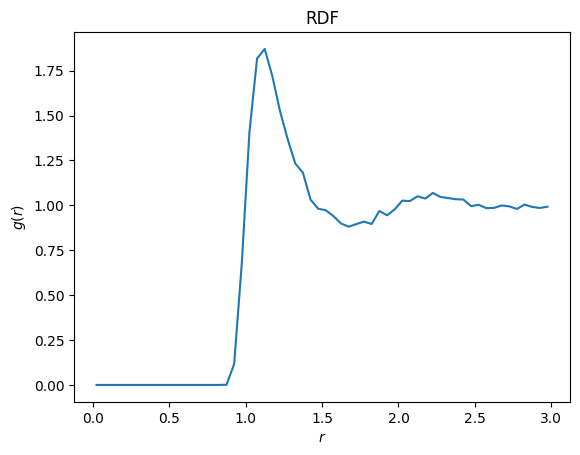
This looks like a typical correlation function for a liquid!